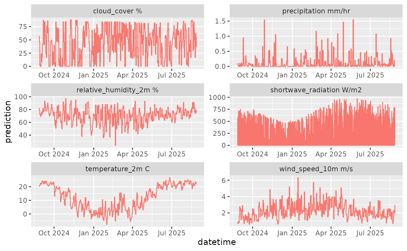
library(ggplot2)
library(dplyr)
library(purrr)
library(tibble)
library(ropenmeteo)
library(lubridate)
library(readr)
Weather forecasts
The open-meteo project combines the best models for each location
across the globe to provide the best possible forecast. open-meteo
refers to this as model = "generic". The maximum forecast
horizon is 16 days.
https://open-meteo.com/en/docs
df <- get_forecast(latitude = 37.30,
                   longitude = -79.83,
                   forecast_days = 7,
                   past_days = 2,
                   model = "generic",
                   variables = c("temperature_2m"))
head(df)
#> # A tibble: 6 × 7
#>   datetime            reference_datetime  site_id   model_id variable prediction
#>   <dttm>              <dttm>              <chr>     <chr>    <chr>         <dbl>
#> 1 2026-06-19 00:00:00 2026-06-21 00:00:00 37.3_-79… generic  tempera…       24.1
#> 2 2026-06-19 01:00:00 2026-06-21 00:00:00 37.3_-79… generic  tempera…       23
#> 3 2026-06-19 02:00:00 2026-06-21 00:00:00 37.3_-79… generic  tempera…       22.8
#> 4 2026-06-19 03:00:00 2026-06-21 00:00:00 37.3_-79… generic  tempera…       21.9
#> 5 2026-06-19 04:00:00 2026-06-21 00:00:00 37.3_-79… generic  tempera…       20.3
#> 6 2026-06-19 05:00:00 2026-06-21 00:00:00 37.3_-79… generic  tempera…       19.6
#> # ℹ 1 more variable: unit <chr>
df |>
  mutate(variable = paste(variable, unit)) |>
  ggplot(aes(x = datetime, y = prediction)) +
  geom_line(color = "#F8766D") +
  geom_vline(aes(xintercept = reference_datetime)) +
  facet_wrap(~variable, scale = "free")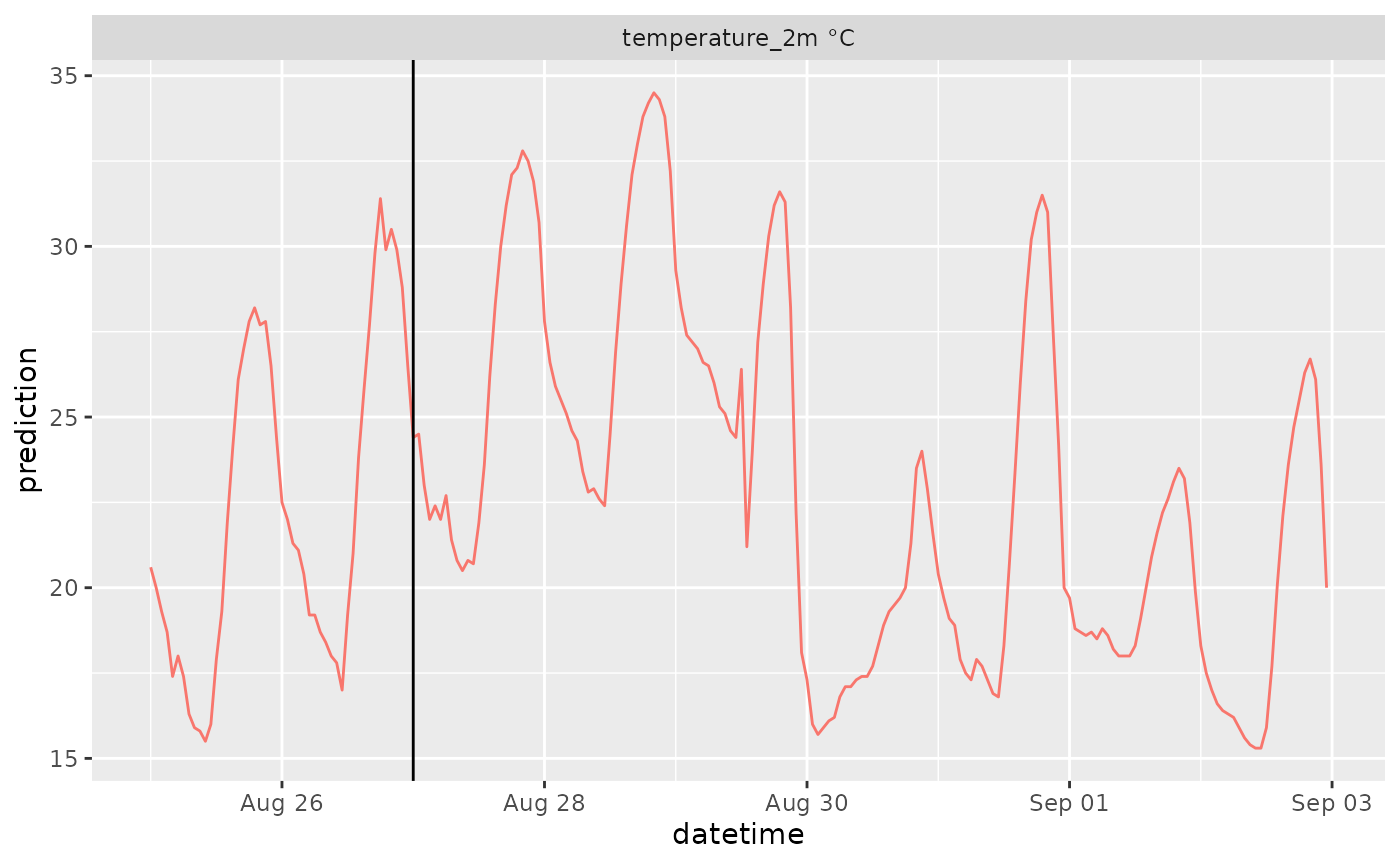
Additional forecast models
Besides "generic", model-specific endpoints are
available. These can be useful when you need a particular agency’s
output or regional high-resolution data.
| Model ID | Agency | Coverage |
|---|---|---|
"gfs" |
NOAA (US) | Global |
"ecmwf" |
ECMWF (EU) | Global, 15 days |
"meteofrance" |
Météo-France | Global/Europe |
"dwd" |
DWD (Germany, ICON) | Global |
"gem" |
Environment Canada | Global, 10 days |
"jma" |
JMA (Japan) | Global, 11 days |
"metno" |
MET Norway | Scandinavia only |
"kma" |
KMA (Korea) | Global, 12 days |
"bom" |
BOM ACCESS-G (Australia) | Global, 7 days |
"ukmo" |
UK Met Office | Global, 7 days |
df_ecmwf <- get_forecast(latitude = 37.30,
                         longitude = -79.83,
                         forecast_days = 7,
                         past_days = 2,
                         model = "ecmwf",
                         variables = c("temperature_2m"))
Ensemble Weather Forecasts
Ensemble forecasts provide probabilistic output from multiple model runs and are available for up to 35 days ahead.
https://open-meteo.com/en/docs/ensemble-api
df <- get_ensemble_forecast(
  latitude = 37.30,
  longitude = -79.83,
  forecast_days = 7,
  past_days = 2,
  model = "gfs_seamless",
  variables = c("temperature_2m"))
head(df)
df |>
  mutate(variable = paste(variable, unit)) |>
  ggplot(aes(x = datetime, y = prediction, color = ensemble)) +
  geom_line() +
  geom_vline(aes(xintercept = reference_datetime)) +
  facet_wrap(~variable, scale = "free", ncol = 2)
Available ensemble models include:
icon_seamless_eps, icon_global_eps, icon_eu_eps, icon_d2_eps,
gfs_seamless_eps, gfs025_eps, gfs05_eps,
ecmwf_ifs025, ecmwf_aifs025,
gem_global, bom_access_global,
ukmo_global_20km, ukmo_uk_2km
Note: ecmwf_ifs025 does not include shortwave
radiation.
Use with the General Lake Model
We have included functions that allow the output to be used with the General Lake Model (https://doi.org/10.5194/gmd-12-473-2019). Since the open-meteo models do not include longwave radiation, the package provides a function to calculate it from cloud cover and air temperature.
glm_variables() returns the variable set required by GLM
for each product and time step:
df <- get_ensemble_forecast(
  latitude = 37.30,
  longitude = -79.83,
  forecast_days = 7,
  past_days = 2,
  model = "gfs_seamless",
  variables = glm_variables(product = "ensemble_forecast",
                            time_step = "hourly"))
head(df)
#> # A tibble: 6 × 8
#>   datetime            reference_datetime  site_id     model_id ensemble variable
#>   <dttm>              <dttm>              <chr>       <chr>    <chr>    <chr>
#> 1 2026-06-19 00:00:00 2026-06-21 00:00:00 37.3_-79.83 gfs_sea… 00       relativ…
#> 2 2026-06-19 00:00:00 2026-06-21 00:00:00 37.3_-79.83 gfs_sea… 01       relativ…
#> 3 2026-06-19 00:00:00 2026-06-21 00:00:00 37.3_-79.83 gfs_sea… 02       relativ…
#> 4 2026-06-19 00:00:00 2026-06-21 00:00:00 37.3_-79.83 gfs_sea… 03       relativ…
#> 5 2026-06-19 00:00:00 2026-06-21 00:00:00 37.3_-79.83 gfs_sea… 04       relativ…
#> 6 2026-06-19 00:00:00 2026-06-21 00:00:00 37.3_-79.83 gfs_sea… 05       relativ…
#> # ℹ 2 more variables: prediction <dbl>, unit <chr>
df |>
  mutate(variable = paste(variable, unit)) |>
  ggplot(aes(x = datetime, y = prediction, color = ensemble)) +
  geom_line() +
  geom_vline(aes(xintercept = reference_datetime)) +
  facet_wrap(~variable, scale = "free", ncol = 2)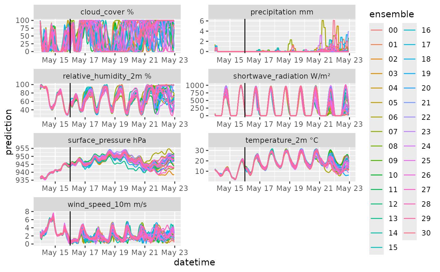
The following converts to GLM format:
path <- tempdir()
df |>
  add_longwave() |>
  write_glm_format(path = path)
head(read_csv(list.files(path = path, full.names = TRUE, pattern = ".csv")[1],
              show_col_types = FALSE))
#> # A tibble: 6 × 7
#>   time                AirTemp ShortWave LongWave RelHum WindSpeed   Rain
#>   <dttm>                <dbl>     <dbl>    <dbl>  <dbl>     <dbl>  <dbl>
#> 1 2026-06-19 00:00:00    22.7        10     426.     72      4.19 0.0336
#> 2 2026-06-19 01:00:00    21           0     414.     81      3.52 0.0336
#> 3 2026-06-19 02:00:00    19.6         0     407.     89      2.78 0.0336
#> 4 2026-06-19 03:00:00    18.6         0     402.     95      2.33 0.0072
#> 5 2026-06-19 04:00:00    18.1         0     402.     97      2.47 0.0072
#> 6 2026-06-19 05:00:00    18           0     401.     96      2.92 0.0072
Converting to Ecological Forecasting Initiative convention
The standard used in the NEON Ecological Forecasting Challenge
differs slightly from this package’s standard. It uses
parameter instead of ensemble because the
Challenge standard accommodates both ensemble (sample) and parametric
distribution forecasts in the same format. The family
column defines the distribution type (here
family = "ensemble").
The EFI standard also follows CF conventions, so variable names are converted to be CF-compliant.
The output from convert_to_efi_standard() matches the
format of neon4cast::stage2(). Learn more at https://projects.ecoforecast.org/neon4cast-docs/Shared-Forecast-Drivers.html.
df |>
  add_longwave() |>
  convert_to_efi_standard()
#> # A tibble: 53,568 × 8
#>    datetime            reference_datetime  site_id     model_id family parameter
#>    <dttm>              <dttm>              <chr>       <chr>    <chr>  <chr>
#>  1 2026-06-19 00:00:00 2026-06-21 00:00:00 37.3_-79.83 gfs_sea… ensem… 00
#>  2 2026-06-19 00:00:00 2026-06-21 00:00:00 37.3_-79.83 gfs_sea… ensem… 00
#>  3 2026-06-19 00:00:00 2026-06-21 00:00:00 37.3_-79.83 gfs_sea… ensem… 00
#>  4 2026-06-19 00:00:00 2026-06-21 00:00:00 37.3_-79.83 gfs_sea… ensem… 00
#>  5 2026-06-19 00:00:00 2026-06-21 00:00:00 37.3_-79.83 gfs_sea… ensem… 00
#>  6 2026-06-19 00:00:00 2026-06-21 00:00:00 37.3_-79.83 gfs_sea… ensem… 00
#>  7 2026-06-19 00:00:00 2026-06-21 00:00:00 37.3_-79.83 gfs_sea… ensem… 00
#>  8 2026-06-19 00:00:00 2026-06-21 00:00:00 37.3_-79.83 gfs_sea… ensem… 00
#>  9 2026-06-19 00:00:00 2026-06-21 00:00:00 37.3_-79.83 gfs_sea… ensem… 01
#> 10 2026-06-19 00:00:00 2026-06-21 00:00:00 37.3_-79.83 gfs_sea… ensem… 01
#> # ℹ 53,558 more rows
#> # ℹ 2 more variables: variable <chr>, prediction <dbl>
Note that neon4cast::stage3() is equivalent to filtering
to the observed period:
df |>
  add_longwave() |>
  convert_to_efi_standard() |>
  filter(datetime < reference_datetime)
#> # A tibble: 11,904 × 8
#>    datetime            reference_datetime  site_id     model_id family parameter
#>    <dttm>              <dttm>              <chr>       <chr>    <chr>  <chr>
#>  1 2026-06-19 00:00:00 2026-06-21 00:00:00 37.3_-79.83 gfs_sea… ensem… 00
#>  2 2026-06-19 00:00:00 2026-06-21 00:00:00 37.3_-79.83 gfs_sea… ensem… 00
#>  3 2026-06-19 00:00:00 2026-06-21 00:00:00 37.3_-79.83 gfs_sea… ensem… 00
#>  4 2026-06-19 00:00:00 2026-06-21 00:00:00 37.3_-79.83 gfs_sea… ensem… 00
#>  5 2026-06-19 00:00:00 2026-06-21 00:00:00 37.3_-79.83 gfs_sea… ensem… 00
#>  6 2026-06-19 00:00:00 2026-06-21 00:00:00 37.3_-79.83 gfs_sea… ensem… 00
#>  7 2026-06-19 00:00:00 2026-06-21 00:00:00 37.3_-79.83 gfs_sea… ensem… 00
#>  8 2026-06-19 00:00:00 2026-06-21 00:00:00 37.3_-79.83 gfs_sea… ensem… 00
#>  9 2026-06-19 00:00:00 2026-06-21 00:00:00 37.3_-79.83 gfs_sea… ensem… 01
#> 10 2026-06-19 00:00:00 2026-06-21 00:00:00 37.3_-79.83 gfs_sea… ensem… 01
#> # ℹ 11,894 more rows
#> # ℹ 2 more variables: variable <chr>, prediction <dbl>
The number of days in the observed period equals
past_days in the call to
get_ensemble_forecast(). The maximum past_days
from open-meteo is 92 days.
Historical Weather
If you need more historical days for model calibration and testing, historical data are available through open-meteo’s ERA5 reanalysis API. ERA5 is available from 1940-01-01 to approximately 5 days before the current date.
https://open-meteo.com/en/docs/historical-weather-api
df <- get_historical_weather(
  latitude = 37.30,
  longitude = -79.83,
  start_date = "2023-01-01",
  end_date = Sys.Date() - lubridate::days(5),
  variables = c("temperature_2m"))
tail(df |> na.omit())
#> # A tibble: 6 × 6
#>   datetime            site_id     model_id variable       prediction unit
#>   <dttm>              <chr>       <chr>    <chr>               <dbl> <chr>
#> 1 2026-06-16 18:00:00 37.3_-79.83 ERA5     temperature_2m       20.9 °C
#> 2 2026-06-16 19:00:00 37.3_-79.83 ERA5     temperature_2m       21.2 °C
#> 3 2026-06-16 20:00:00 37.3_-79.83 ERA5     temperature_2m       21.1 °C
#> 4 2026-06-16 21:00:00 37.3_-79.83 ERA5     temperature_2m       21.1 °C
#> 5 2026-06-16 22:00:00 37.3_-79.83 ERA5     temperature_2m       21.4 °C
#> 6 2026-06-16 23:00:00 37.3_-79.83 ERA5     temperature_2m       20.6 °C
df |>
  mutate(variable = paste(variable, unit)) |>
  ggplot(aes(x = datetime, y = prediction)) +
  geom_line(color = "#F8766D") +
  geom_vline(aes(xintercept = lubridate::with_tz(Sys.time(), tzone = "UTC"))) +
  facet_wrap(~variable, scale = "free")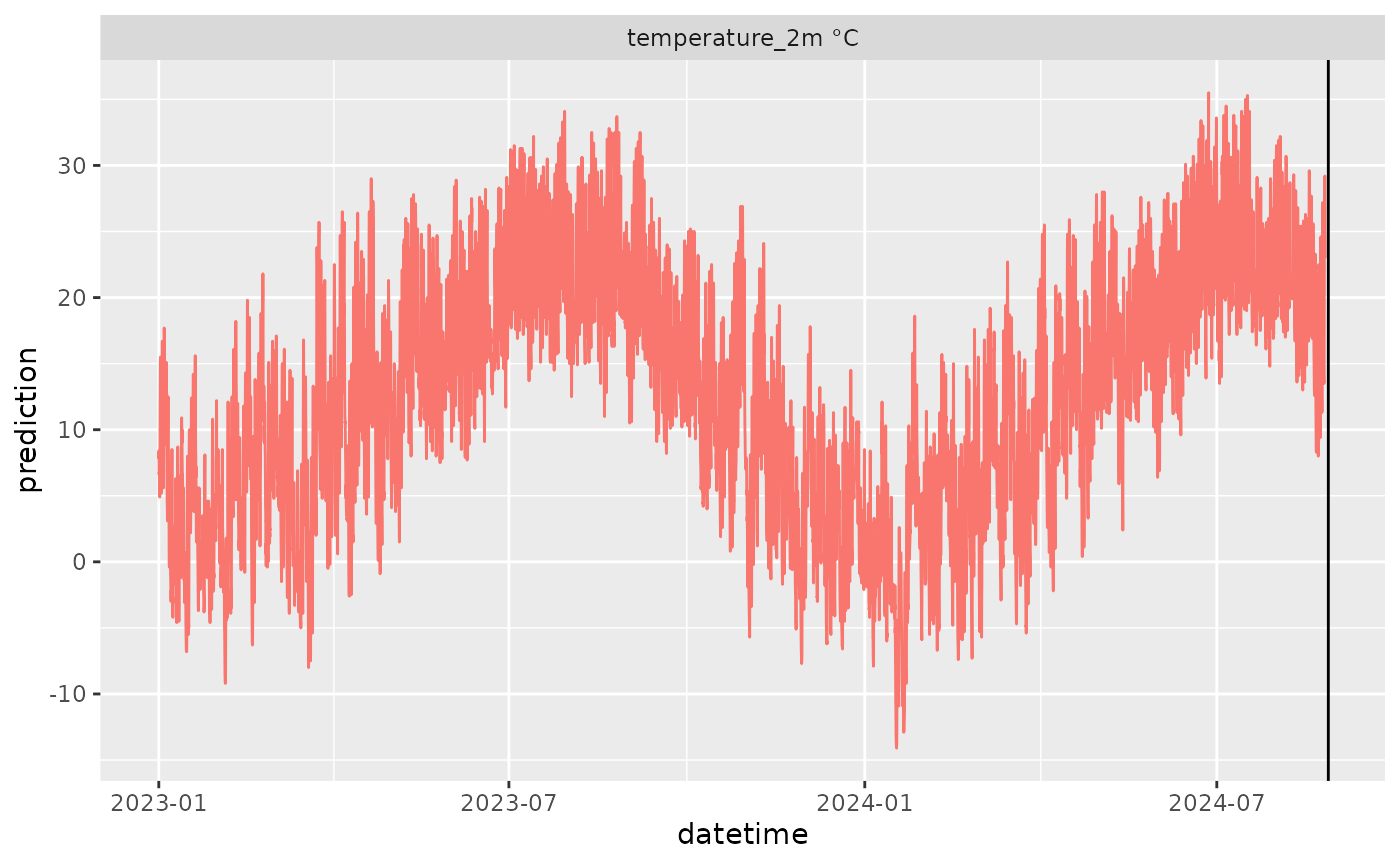
Seasonal Forecasts
Seasonal forecasts covering up to 7 months ahead are provided by
ECMWF. The default "ecmwf_seasonal_seamless" model blends
EC46 (updated daily, 46-day horizon) with SEAS5 (updated monthly,
7-month horizon) for the best available coverage at any lead time.
https://open-meteo.com/en/docs/seasonal-forecast-api
df <- get_seasonal_forecast(
  latitude = 37.30,
  longitude = -79.83,
  forecast_days = 30,
  past_days = 5,
  variables = c("temperature_2m"))
head(df)
#> # A tibble: 6 × 8
#>   datetime            reference_datetime  site_id     model_id ensemble variable
#>   <dttm>              <dttm>              <chr>       <chr>    <chr>    <chr>
#> 1 2026-06-16 00:00:00 2026-06-21 00:00:00 37.3_-79.83 ecmwf_s… 00       tempera…
#> 2 2026-06-16 00:00:00 2026-06-21 00:00:00 37.3_-79.83 ecmwf_s… 01       tempera…
#> 3 2026-06-16 00:00:00 2026-06-21 00:00:00 37.3_-79.83 ecmwf_s… 02       tempera…
#> 4 2026-06-16 00:00:00 2026-06-21 00:00:00 37.3_-79.83 ecmwf_s… 03       tempera…
#> 5 2026-06-16 00:00:00 2026-06-21 00:00:00 37.3_-79.83 ecmwf_s… 04       tempera…
#> 6 2026-06-16 00:00:00 2026-06-21 00:00:00 37.3_-79.83 ecmwf_s… 05       tempera…
#> # ℹ 2 more variables: prediction <dbl>, unit <chr>
df |>
  mutate(variable = paste(variable, unit)) |>
  ggplot(aes(x = datetime, y = prediction, color = ensemble)) +
  geom_line() +
  geom_vline(aes(xintercept = reference_datetime)) +
  facet_wrap(~variable, scale = "free")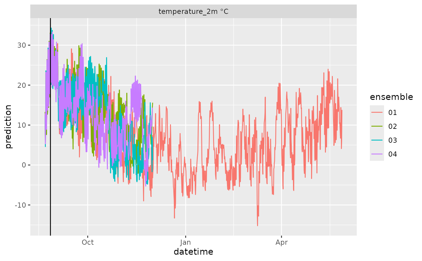
Downscaling from 6-hourly to hourly time step
The seasonal API delivers data at 6-hourly intervals. The package
provides six_hourly_to_hourly() to downscale to hourly
using linear interpolation for most variables and solar geometry for
shortwave radiation.
df <- get_seasonal_forecast(
  latitude = 37.30,
  longitude = -79.83,
  forecast_days = 30,
  past_days = 5,
  variables = glm_variables(product = "seasonal_forecast",
                            time_step = "6hourly"))
df |>
  six_hourly_to_hourly(latitude = 37.30, longitude = -79.83,
                       use_solar_geom = TRUE) |>
  mutate(variable = paste(variable, unit)) |>
  ggplot(aes(x = datetime, y = prediction, color = ensemble)) +
  geom_line() +
  geom_vline(aes(xintercept = reference_datetime)) +
  facet_wrap(~variable, scale = "free", ncol = 2)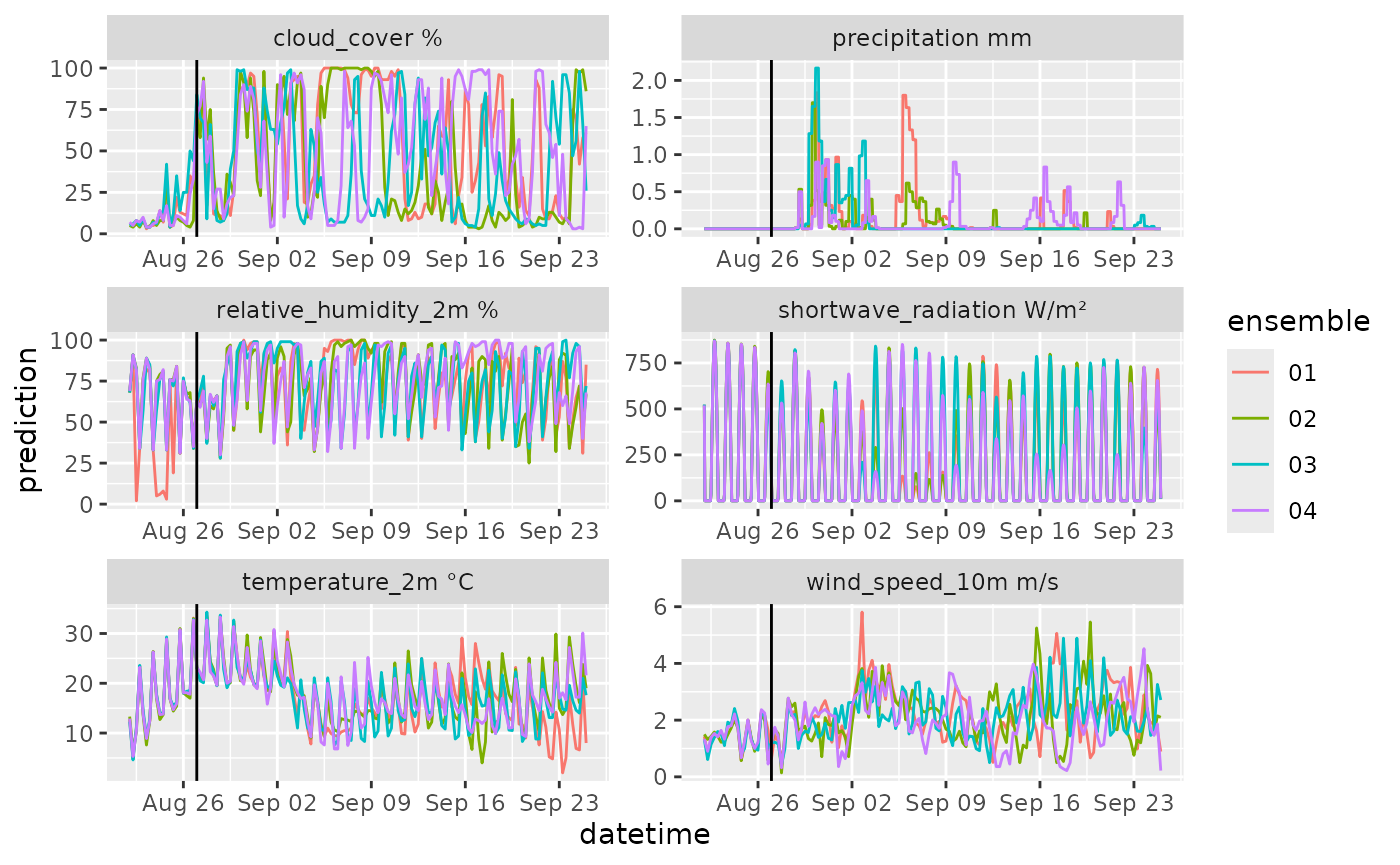
Climate Projections
Daily climate projections from seven high-resolution CMIP6 models are available from 1950 through 2050.
Note that shortwave radiation units differ from the forecast APIs:
the climate API returns shortwave_radiation_sum in MJ/m²
(daily total) rather than instantaneous W/m².
https://open-meteo.com/en/docs/climate-api
df <- get_climate_projections(
  latitude = 37.30,
  longitude = -79.83,
  start_date = Sys.Date(),
  end_date = Sys.Date() + lubridate::years(1),
  model = "EC_Earth3P_HR",
  variables = c("temperature_2m_mean"))
head(df)
#> # A tibble: 6 × 6
#>   datetime   site_id     model_id      variable            prediction unit
#>   <date>     <chr>       <chr>         <chr>                    <dbl> <chr>
#> 1 2026-06-21 37.3_-79.83 EC_Earth3P_HR temperature_2m_mean       18.7 °C
#> 2 2026-06-22 37.3_-79.83 EC_Earth3P_HR temperature_2m_mean       20.1 °C
#> 3 2026-06-23 37.3_-79.83 EC_Earth3P_HR temperature_2m_mean       20.7 °C
#> 4 2026-06-24 37.3_-79.83 EC_Earth3P_HR temperature_2m_mean       21.3 °C
#> 5 2026-06-25 37.3_-79.83 EC_Earth3P_HR temperature_2m_mean       22.4 °C
#> 6 2026-06-26 37.3_-79.83 EC_Earth3P_HR temperature_2m_mean       23.1 °C
df |>
  mutate(variable = paste(variable, unit)) |>
  ggplot(aes(x = datetime, y = prediction)) +
  geom_line(color = "#F8766D") +
  facet_wrap(~variable, scale = "free")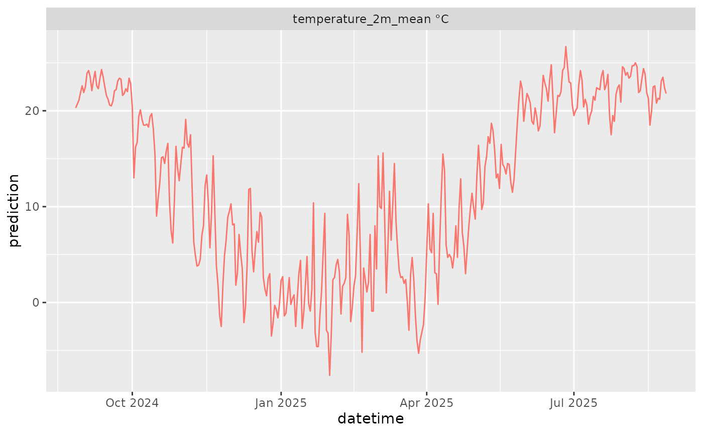
Downloading multiple sites or models
Multiple models
models <- c("CMCC_CM2_VHR4", "FGOALS_f3_H", "HiRAM_SIT_HR",
            "MRI_AGCM3_2_S", "EC_Earth3P_HR", "MPI_ESM1_2_XR", "NICAM16_8S")

df <- map_df(models, function(model) {
  get_climate_projections(
    latitude = 37.30,
    longitude = -79.83,
    start_date = Sys.Date(),
    end_date = Sys.Date() + lubridate::years(1),
    model = model,
    variables = c("temperature_2m_mean"))
})
df |>
  mutate(variable = paste(variable, unit)) |>
  ggplot(aes(x = datetime, y = prediction, color = model_id)) +
  geom_line() +
  facet_wrap(~variable, scale = "free")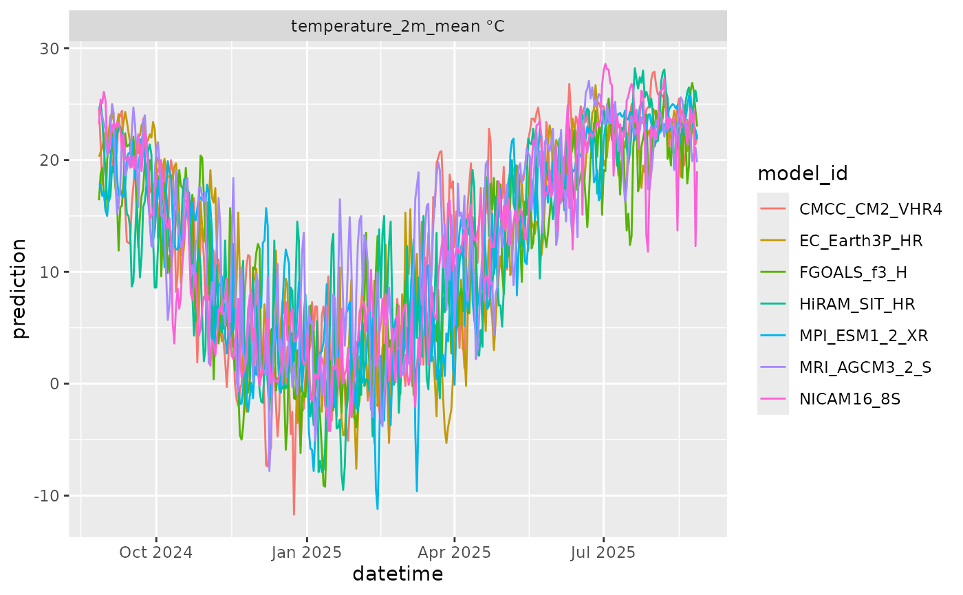
Multiple sites
The optional site_id argument labels rows for each
location, making it easy to combine results from multiple sites.
sites <- tibble(site_id = c("fcre", "sunp"),
                latitude = c(37.30, 43.39),
                longitude = c(-79.83, -72.05))

df <- map_df(1:nrow(sites), function(i, sites) {
  get_climate_projections(
    latitude = sites$latitude[i],
    longitude = sites$longitude[i],
    site_id = sites$site_id[i],
    start_date = Sys.Date(),
    end_date = Sys.Date() + lubridate::years(1),
    model = "MPI_ESM1_2_XR",
    variables = c("temperature_2m_mean"))
}, sites)
head(df)
#> # A tibble: 6 × 6
#>   datetime   site_id model_id      variable            prediction unit
#>   <date>     <chr>   <chr>         <chr>                    <dbl> <chr>
#> 1 2026-06-21 fcre    MPI_ESM1_2_XR temperature_2m_mean       23.8 °C
#> 2 2026-06-22 fcre    MPI_ESM1_2_XR temperature_2m_mean       24.3 °C
#> 3 2026-06-23 fcre    MPI_ESM1_2_XR temperature_2m_mean       24.7 °C
#> 4 2026-06-24 fcre    MPI_ESM1_2_XR temperature_2m_mean       25.8 °C
#> 5 2026-06-25 fcre    MPI_ESM1_2_XR temperature_2m_mean       25.2 °C
#> 6 2026-06-26 fcre    MPI_ESM1_2_XR temperature_2m_mean       24.5 °C
df |>
  mutate(variable = paste(variable, unit)) |>
  ggplot(aes(x = datetime, y = prediction, color = site_id)) +
  geom_line() +
  facet_wrap(~variable, scale = "free")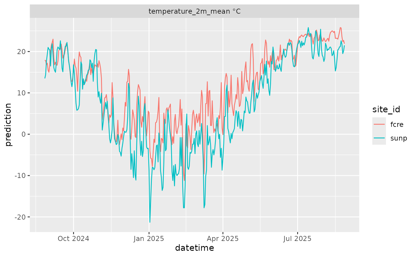
Converting from daily to hourly time step
Photosynthesis responds non-linearly to shortwave radiation, so
applying a daily mean to every hour underestimates peak midday
production. daily_to_hourly() uses solar geometry to
redistribute the daily radiation total across daylight hours, and
divides precipitation sums evenly across 24 hours. All other variables
have their daily mean applied to each hour.
df <- get_climate_projections(
  latitude = 37.30,
  longitude = -79.83,
  start_date = Sys.Date(),
  end_date = Sys.Date() + lubridate::years(1),
  model = "EC_Earth3P_HR",
  variables = glm_variables(product = "climate_projection", time_step = "daily"))
#> Waiting 3s for throttling delay ■■■■■■■■■■
#> Waiting 3s for throttling delay ■■■■■■■■■■■■■■■■■■■■■■■■■■
#> Waiting 3s for throttling delay ■■■■■■■■■■■■■■■■■■■■■■■■■■■■■■
#> Waiting 6s for throttling delay ■■■■■■■■■■
#> Waiting 6s for throttling delay ■■■■■■■■■■■■■■■■■■■■■■■■■
#> Waiting 6s for throttling delay ■■■■■■■■■■■■■■■■■■■■■■■■■■■■■■■
#> Waiting 5s for throttling delay ■■■■■■
#> Waiting 5s for throttling delay ■■■■■■■■■■■■■■■■■■■■■■■
#> Waiting 5s for throttling delay ■■■■■■■■■■■■■■■■■■■■■■■■■■■■■■■
#> Waiting 5s for throttling delay ■■■■■■
#> Waiting 5s for throttling delay ■■■■■■■■■■■■■■■■■■■■■■■
#> Waiting 5s for throttling delay ■■■■■■■■■■■■■■■■■■■■■■■■■■■■■■■
#> Waiting 5s for throttling delay ■■■■■■■■■■
#> Waiting 5s for throttling delay ■■■■■■■■■■■■■■■■■■■■■■■■■■■■
#> Waiting 5s for throttling delay ■■■■■■■■■■■■■■■■■■■■■■■■■■■■■■■
df |>
  daily_to_hourly(latitude = 37.30, longitude = -79.83) |>
  mutate(variable = paste(variable, unit)) |>
  ggplot(aes(x = datetime, y = prediction)) +
  geom_line(color = "#F8766D") +
  facet_wrap(~variable, scale = "free", ncol = 2)